We take estimates of population from Marcus and Flannery [Flan96] and fit these to three models.
Approach 1: A Simple Growth Function . The simplest possible model is to ignore all limitations on growth, such as resources, disease, warfare etc. and calculate the population of each succeeding generation assuming a constant average number of surviving children per breeding pair. If we assume a granfather-father-son structure of the population, then we can set the fraction of breeding pairs at one sixth of the population (one third of the population is producing children). If we again assume that one third of each generation die, then the population of the next generation is given by

Where “n” is the previous population and “k” is average number of surviving children produced by a breeding pair.
Let us assume we are looking at a total population of 5280 at the end of the third generation, and that this figure is 5 times the intial population, i.e. the initial population was a feasible n = 1056. Assuming three generations per century, then if each breeding pair on average produces k = 6.26 surviving children, the population figures for each succeeding generation from Equation 1 are, after 1 generation, 1.710n = 1805.76, after two generations 2.924n = 3087.74 and after 3 generations (i.e.100 years, 400 BC) 5.000n = 5280.00. The average of over 6 surviving children per pair is extremely high, and reducing the initial population only makes it higher, while increasing the initial population demands a move of over 50% of the entire population to the remote hill-top of Monte Albán. On the basis of this very simple model it appears highly likely that fairly continuous immigration to the Monte Albán hilltop must have been the primary mechanism for population growth.
In this modeling exercise we have completely ignored any restrictions on population growth, and assumed the population can grow indefinitely. Extrapolating this growth to 9 generations (i.e. to 200BC) yields a population of 132,017, far in excess of the estimated 17,000 [ref.]. It is clear that we cannot ignore population restricting factors during the Monte Albán epoch, and in the next models we implicitly include such restraints.
Approach 2: A Simple Growth Function with Limitations . This model is the simplest possible which includes a limit to growth, and involves only the average number of surviving children per breeding pair of the population. Provided it remains constant, the fraction of the population of breeding age does not enter into the model. The only estimate required is the average generation gap, and many genealogical studies have indicated that three generations per century is a remarkably good approximation [ref.]. The model assumes that the population grows by consuming a fixed supply of resources, and reduces to the simple equation:
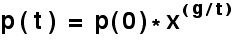
Where “p(0)” is the starting population at time “t=0”, “g” is the generation period in years, and “p(t)” the population after “t” years. The factor “x” is the breeding factor such that the average number of surviving children per breeding pair is “2x”. The analysis is presented in Table 1. This model assumes that population is generated out of resources, and that when resources are exhausted, growth stops. [1]
Table 1. Populations of San José Mogote and Monte Albán I
| Epoch | Approximate Date (BC) | Population | Time Interval, “t”, (years) | Breeding Factor, “x” | Calculated Population “p(t)” from Equation 2 | Mean Number of Children per Breeding Pair |
|---|---|---|---|---|---|---|
| Population figures are taken from [Flan96]. | ||||||
| San José Mogote at end of Rosario period | 500 | 2,000 | 0 | - | - | - |
| Monte Albán I, early | 400 | 5,280 | 100 | 1.382 | 5,279 | 2.764 |
| Monte Albán I, late | 200 | 17,000 | 300 | 1.2685 | 17,007 | 2.537 |
The breeding factors in the table are those required to fit the population estimates by Marcus and Flannery, [Flan96]. The most obvious point is that these breeding factors are very high (1.27-1.38), modern estimates for Europe and the USA are of the order of 1.05. Assuming a population growth from some small value, perhaps 200, in 1600 BC to 2,000 in 500 BC yields a much more normal breeding factor of only 1.095. Clearly, at the end of the Rosario period there occurred a period of unusually rapid growth, with most families producing many surviving children. Some external factor must have influenced this onset of rapid growth.
This model takes no account of any possible growth of resources.
Approach 3. A Realistic Logistic Approach . Modern studies of population growth take account of the self-limiting nature of population growth. Approach 1 above predicts that population will continue to grow indefinitely, while Approach 2 permits growth until resources are exhausted. Whilst these might be adequate for growth in its early stages, they are unrealistic during later stages or when the resources available to the population are in any way variable. More sophisticated attempts at modeling growth either assume a functional form which insists upon a levelling off without any specific assumptions that resources are the limiting factor. It is often appropriate to express these functions in a logistic form in which each successive step in population growth is calculated from its previous value. The models all require adjustable parameters to fit observations or estimates of population values.
Parametric Models for Growth . The general form of population growth is an initial period of slow growth, followed by a period of rapid, possibly exponential growth, until finally other factors, such as depletion of resources, lead to a tailing off of growth and an approach to a limiting level. This sigmoidal form can be represented by continuous functions such as the Gompertz growth curve.
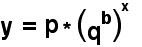
Where “b”, “p” and “q” are adjustable parameters. The Gompertz curve is sometimes extended with an additional parameter added on to Equation 3. An alternative growth equation is the Pearl-Reed logistic curve.
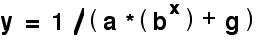
Where “a”, “b” and “g” are the adjustable parameters. These growth functions are all capable of producing acceptable aggreement with the observed populations at 400 and 200 BC, for example the Pearl-Reed function
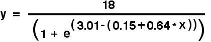
gives values of y=1.0 at x=0, y=5.2 at x=3, and y=17.02 at x=9. [[*** note these are thousands of population, I ought to give a solution for actual populations ***]]
However, it is more natural to think of population growth as a stepwise process, with each generation producing the next, and a transformation of the logistic function leads to the simple growth function investigated extensively and applied by Robert May [May76] to population growth. [2]
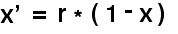
Each succeeding value of the population, “x'”, is calculated from the previous value, “x” using a constant growth rate factor, “r”. In this form population can, in principle, vary from some initial value, x > 0, up to unity, but will generally level off at some intermediate value, 0 < x < 1. It is natural, but not necessary, to identify each step with a generation, and the leveling off of population below the maximum conceivable population (unity) with the influence of factors such as limited resources, internal or external conflict etc. As it stands Equation 6 requires only estimates of the initial population and the growth rate factor. However, a third parameter is required to scale the output to real population figures.
It appears from the available evidence that Monte Albán was initially populated around 500 BC by a transfer of peoples from other settlements in the valley of Oaxaca [ref]. There is no direct evidence of the number of people involved in the initial settlement, but it would have been very unlikely to have exceeded half of the total population of the valley at the end of the Rosario period (about 2000 ???), and must have been large enough to produce a successful on-going growth at the new site (perhaps a minimum of around 100). The settlement obviously prospered, and by 400 BC the population has been estimated at around 5,200 [ reference needed ]. Rapid growth continued, and by 200 BC it had reached about 17,000 [ref.]. By any standards this would be an extremely rapid growth of population if one were to attribute the growth solely to breeding internal to the population, and almost certainly the population was swelled by further and continuous immigration from other small settlements in the surrounding valley.
We have used the logistic growth of Equation 6, combined with two population estimates of 5,200 at 400 BC and 17,000 at 200 BC to estimate the initial influx of population at the Monte Albán site, and to predict future growth. We find four possible solutions that agree with the population estimates at 400 and 200 BC. To scale the growth to a real time basis we assume three steps or generations per century. Three parameters are required to accomplish the fit: the initial population, the growth rate factor, and a “maximum conceivable population”. This last parameter is required to scale Equation 6 from the range 0<x<1 to real population figures.
Statistical Confidence . The question arises of the reliability of the solutions obtained. The most commonly used statistic for curve fitting of this type is the reduced chi-square test statistic,

where each “resid” is given by the difference between the population estimate and the calculated value from the model. “chi-sq” is not always adequate [Cat83], but more and better population data would be required for more sophisticated analysis. In Equation 7, “n” is the number of points to be fitted, and “p” the number of adjustable parameters. It is immediately obvious that we cannot calculate this statistic directly from the Monte Albán population data since we have p > n. In other words, we need more population data to produce a real statistic.
However, we can compute and minimize the sum of the squared residuals for a given set of the three parameters, confident that as this sum approaches zero we have a good fit to the population data, ideally perfect when the sum of squared residuals is zero. We might expect to find an infinite number of solutions to this over-parameterized curve fitting process, but, perhaps rather surprisingly, we only find the four solutions which are detailed below in the following tables.
Table 2. Model A, Initial Population 436
| Generation | Date (BC) | Population |
|---|---|---|
| 0 | 500 | 436.0 |
| 1 | 467 | 1026.5 |
| 2 | 433 | 2367.3 |
| 3 | 400 | 5200.2 |
| 4 | 367 | 10220.1 |
| 5 | 333 | 15896.1 |
| 6 | 300 | 17356.1 |
| 7 | 267 | 16880.9 |
| 8 | 233 | 17073.8 |
| 9 | 200 | 16999.9 |
| Sum of residuals squared = 0.05900 | ||
| Initial Population = 436.0 | ||
| Growth rate factor = 2.39 | ||
| Population after 3 generations (100 years, 400 BC) = 5200.2 | ||
| Population after 9 generations (300 years, 200 BC) = 16999.9 | ||
Table 3. Model B, Initial Population 840
| Generation | Date (BC) | Population |
|---|---|---|
| 0 | 500 | 840.0 |
| 1 | 467 | 1586.6 |
| 2 | 433 | 2931.6 |
| 3 | 400 | 5200.0 |
| 4 | 367 | 8574.9 |
| 5 | 333 | 12548.6 |
| 6 | 300 | 15621.4 |
| 7 | 267 | 16806.7 |
| 8 | 233 | 16986.3 |
| 9 | 200 | 17000.1 |
| Sum of residuals squared = 0.00779 | ||
| Initial Population = 840.0 | ||
| Growth rate factor = 1.935 | ||
| Population after 3 generations (100 years, 400 BC) = 5200.0 | ||
| Population after 9 generations (300 years, 200 BC) = 17000.1 | ||
Table 4. Model C, Initial Population 1069
| Generation | Date (BC) | Population |
|---|---|---|
| 0 | 500 | 1068.7 |
| 1 | 467 | 1859.1 |
| 2 | 433 | 3165.9 |
| 3 | 400 | 5200.0 |
| 4 | 367 | 8051.5 |
| 5 | 333 | 11404.2 |
| 6 | 300 | 14383.6 |
| 7 | 267 | 16158.3 |
| 8 | 233 | 16824.9 |
| 9 | 200 | 17000.0 |
| Sum of residuals squared = 0.00046 | ||
| Initial Population = 1068.7 | ||
| Growth rate factor = 1.789 | ||
| Population after 3 generations (100 years, 400 BC) = 5200.0 | ||
| Population after 9 generations (300 years, 200 BC) = 17000.0 | ||
Table 5. Model D, Initial Population 1365
| Generation | Date (BC) | Population |
|---|---|---|
| 0 | 500 | 1364.5 |
| 1 | 467 | 2180.5 |
| 2 | 433 | 3418.0 |
| 3 | 400 | 5199.8 |
| 4 | 367 | 7564.4 |
| 5 | 333 | 10335.9 |
| 6 | 300 | 13052.6 |
| 7 | 267 | 15158.6 |
| 8 | 233 | 16411.7 |
| 9 | 200 | 17000.1 |
| Sum of residuals squared = 0.03616 | ||
| Initial Population = 1364.5 | ||
| Growth rate factor = 1.649 | ||
| Population after 3 generations (100 years, 400 BC) = 5199.8 | ||
| Population after 9 generations (300 years, 200 BC) = 17000.1 | ||
Modeling Procedures . The minimization procedure consisted first of a wide but finely meshed scan of the whole 3-dimensional parameter space.
The initial population parameter was scanned from 250 to 1500 in steps of 5.
The growth rate factor was scanned from 1.5 to 2.8 in steps of 0.01.
The “maximum conceivable population” parameter was scanned from 17,000 to 50,000 in steps of 100.
The resulting list of summed squared residuals was sorted and scanned for low values indicating proximity to a solution. In subsequent phases the scans of the parameter space were progressively confined to the region of the suspected solutions until the sum of squared residuals was below 0.06, and the fit to the populations at 400 and 200 BC was good to within ±0.2.
In the next phase, the generation to generation growth was calculated for each of the four solutions found. The results are shown in Figure 1. below.
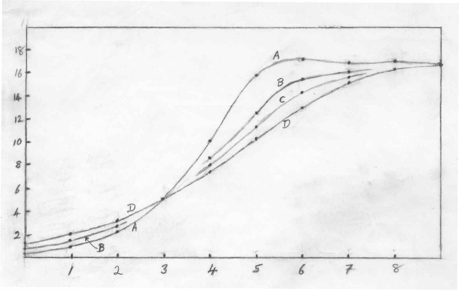
Discussion . The four solutions, which we label A, B, C and D, in Figure 1, correspond to Table 2, Table 3, Table 4 and Table 5 respectively, and all show the expected sigmoidal form, a slow initial growth, a period of rapid growth, and a leveling off. There is no information derived from the modeling process which suggests even a preference for any one of the four solutions. There are some general observations we can make that are of significance to the problem of population growth in Monte Albán I.
Fractional population figures have no meaning - they are an artifact produced by the requirement to reduce the sum of squared residuals to below 0.06.
All the models show that it was possible for a relatively small settlement (of the order of 200 to 1500) to grow to the population estimates suggested for 100 and 300 years later. However, see considerations below which suggest that this could not be solely internal expansion of population, and that immigration is required.
All the models predict a leveling off of population at around the 17,000 mark after about 200-250 years at 400 to 350 BC, and that the calculated population later remains constant for up to 25 generations at least (around 300 AD)
Perhaps the most significant result of this modeling is the leveling off of population. The functional form of Equation 6 requires that in order to fit the data the population must level off at 17,000. In order for the population to exceed this value there must have occurred a significant change in the external environment: given the resources available in Monte Albán I, the population has reached its optimum level. Only by changing the resources will Equation 6 permit further growth.
The first fortifications appear at Monte Albán appear at about 300 BC, and are consistent with the growth of a significant external threat, with warfare limiting the population.
The leveling off at 17,000 is also consistent with a population limited by available resources, perhaps awaiting the development of new agricultural techniques to increase resources (e.g. new irrigation techniques to raise the productivity of sem-arid terraces).
The limit of population growth from Equation 6, together with the onset of fortifications implies that Monte Albán had by this rime become a rich site atractive to aggressors, and that raiding was more immediately productive than immigration. Presumably the aggressors were he other, growing settlements in the vally, perhaps motivated by a growinf resentment of the requirement to provision the hill-top site. Push a sub-servient population too hard and it will rebel. [3]
Model A, with the smallest initial settlement (436) requires a very high rate of population increase from about 400 to 300 BC, when the population increases almost linearly at a rate of over 4,000 per generation from 5,200 at 400 BC to 17356 at 300 BC. During the first generation following 400 BC, the population doubles. This we feel is a very unrealistic rate for an internal population growth, if one third of the population die in each generation, and only one third are producing children are producing children, they would be required to produce an average of 8.00 surviving children per breeding pair. We conclude that Model A must imply very considerable immigration into Monte Albán.
We also observe in Model A, an overshoot in population at 300 BC followed by convergent oscillation to the limiting population of 17,000. Such oscillations are typical of situations of high growth rate, and although reasonable, their magnitude is far too small to be susceptible to verification.
At the other end of the scale, Model D, with a much larger initial population (1365) shows a much slower and steadier population growth, but it is still very high. Making the same assumptions about death rate and fraction of breeding population leads to a requirement of 4.83 surviving children per breeding pair. We consider this to be also highly improbable and again conclude again that considerable immigration to Monte Albán must have been responsible for the estimated increase in population [ref.].
[[[***** a word of explanation, probably not suitable for publication. Model A: population at 400 BC was 5,200, of these about 1/3 are pre-breeding age, 1/3 of breeding age, and 1/3 post-breeding age. The 1/3 post-breeding age die during the generation. The population after one generation in 367 BC predicted by Model A is 10220 (see Table 2), an increase of 5020, but we have also lost 1673 (1/3 of 5,200) by death, so the total number of children required to raise the population to 10220 would be 6693 (5020+1673), and these must be produced by 836 (1673/2) breeding pairs, or an average of 8.00 surviving children per breeding pair. Similarly, for Model D we require 4.83 surviving children required per breeding pair. It is possible (likely?) that life expectancy was low, and that the fraction of the population of post-breeding age was much lower than 1/3. This would effectively increase the breeding population fraction and reduce the average numbers of surviving children per breeding pair. In the extreme limit of no post-breeding population, and 2/3 of the population producing children, the figures reduce to 4.00 for Model A and 2.46 for Model D. (This still assumes that 1/3 of the population die in each generation - I don't see how we can avoid that.) An average of 4 surviving children per pair is still an unrealistically high average, and considerable immigration is still required. For Model D, 2.46 is still high (compare modern figures of around 2.1 for rapidly developing countries), but feasible, and we might not be able to infer much immigration. *****]]]
Models B and C lie intermediate between A and D (not surprisingly), and lead to similar estimates of child producing capacity of 6.86 and 6.28 respectively [[***check these figures***]]. Both of these rates are unacceptably high and also favor considerable immigration to Monte Albán in the period 500 to 200 BC.
This simple logistic treatment ignores the fact that resources will generally be themselves subject to growth and depletion (consider the deer population in the valley of Oaxaca as the human population grows). More sophicated modelling of population, still based on the logistic approach, include the effect of a growing population upon its environment. With the very limited human population data available for Monte Albán, and the almost total lack of any real estimates of animal and vegetable resources, more sophisticated analysis is impossible.
It is interesting to comapre the growth of population at Monte Albán I in the century 500-400 BC with the growth of the modern city of Oaxaca over the last 100 tears when the population increased from about 30,000 to 300,000. [4] The average increase per year in the twentieth century was 2,700, and the average percentage based on the average population this period is 1.637% per year, which compares quite favorably with the value of 0.86% per year found in Section 1 for Monte Albán I. Assuming three generations per century, and an initial population of 30,000, then if each breeding pair on average produces k = 8.9267 surviving children, the population figures for each succeeding generation from Equation 1 are, after 1 generation, 64,634, after two generations 139,250 and after 3 generations (i.e.100 years) 300,006. There can be little doubt that the major factor in the growth of the modern city of Oaxaca has been immigration - the drift from the surrounding land to the central city, probably significantly enhanced by immigration from further afield.
Conclusions . The overall picture of settlement at Monte Albán is of a small, confident initial population at 500 BC, under no significant external threat, with more than adequate resources, breeding rapidly and attracting immigration from other villages for about 200 years. Somewhere around 300 BC there arose an external threat sufficiently serious to make fortification necessary and to stop expansion both by warfare and discouraging immigration.
It is of interest to extend this modeling to later expansion at Monte Albán when we must infer that the external threat was overcome, warfare effectively ceased, and once more Monte Albán became attractive to immigrants (availability of work, both building and supplying food to a growing population.)
[1] This model is essentially the first order rate equation in chemical kinetics.
[2] The logistic function explored by May [May76] displays some remarkable features which lead to some of the earliest studies of “chaos” in mathematical systems. These effects only occur when the growth rate factor “r” exceeds 3.0, but can lead to wide and random fluctuations, and even to complete collapse of populations. It is interesting to speculate if the collapse of many civilizations, including the Zapotecs at Monte Albán, in the post-classic epoch followed a period of exceptionally high population growth. James Gleick [Gleick86] is an easy introduction to chaotic systems.
[3] Perhaps this is what happened earlier at San José Mogote when a splinter group broke off to settle Monte Albán.
[4] The precision of these modern figures for Oaxaca city is scarcly any better than those for Monte Albán I.