Table of Contents
- Nuclear Properties
- Electronic Properties
- Neutron Activation Analysis
- Acid Extraction
- Morphological Inspection
- Comparisons
- Identification of Sources
- Rocks or Pots
- Errors or Features
- Complimentary Techniques
- Statistics
- Model Fitting to Data
- Conclusions
- Some final thoughts on cluster analysis.
- Ron Catterall, 29 August 2005
Chemical elements are distinguished from each other by the count of protons in the atomic nucleus: the aluminum atom is characterized by 13 protons (and 14 neutrons) in its nucleus. If a given nucleus contains only 12 protons it is calcium. An atomic nucleus is only stable if the ratio of protons to neutrons lies within certain, largely empirical, limits. Outside these limits the nucleus will spontaneously decay, generally with the emission of particles and/or quanta of energy. Adding an extra neutron to a nucleus (as in neutron activation analysis) can tip the balance between stability and radioactivity..
The chemical environment of an atom is distinguished by the form of the electronic wave function of the extra nuclear electrons of the atom: somewhat crudely, the distribution of electrons around the nucleus. The aggregation of atoms into molecular species (such as naturally occurring minerals) involves major restructuring of the distribution of the most loosely bound electrons and a new chemical environment. This chemical environment is responsible for chemical properties such as acid solubility. Annealing or firing processes will generally result in changes of chemical environment.
An atomic nucleus can exist in a variety of distinct (quantized) energy states, and is normally found in its lowest energy state (the ground state). The technique of neutron activation analysis (NAA) consists in promoting the nucleus of an atom to a higher energy state by bombarding it with neutrons to produce a very short-lived (10-13 sec.) excited nuclear state in which an additional neutron is incorporated into the nucleus of the stable atomic target. The nucleus in this excited state generally has several possible methods of returning to the ground state. These can include the production of other isomeric forms (either stable or radioactive) of the nucleus, different atomic species (transmutation of elements, the philosopher’s stone), or a return to the original nuclear form. The one of interest to us is the inelastic scattering process in which a neutron of different energy is emitted accompanied by a (usually gamma) photon. The energies of this photon and the secondary neutron are characteristic of the composition of the nucleus and serve to identify its chemical nature. The emitted particles are almost completely independent of the electronic wave function of the extra-nuclear electrons, that is, of its chemical environment. The number of quanta emitted is a measure of the number of atoms in the sample under investigation and can, at least in principle, be calculated directly knowing the cross section for neutron capture and the characteristics of the irradiating neutron beam. In practice such absolute determinations are generally replaced by comparisons with scattering data from standard known samples. Basically INAA counts atomic nuclei for distinct chemical atoms independent of their chemical environment. It is not sensitive enough to distinguish between chemical (molecular) environments of the atom. (Other techniques such as electron spin resonance can detect changes in the electronic wave function of atoms due to the presence of additional neutrons in the nucleus – ref. Catterall and Edwards, Phil. Mag.(?) ca. 1982.)
(Elastic neutron scattering in which the irradiating neutrons effectively bounce off the target nuclei unchanged, but in preferred directions can give details of the environment of the nucleus such as the crystalline form, but as far as I am aware this has not been attempted so far for complex archaeological samples, it normally requires single crystal samples. See work of Catterall, Chieux, Damay and Glaunsinger at ILL, Grenoble on the structure of calcium hexammine – ref. approx. 1984, probably J. Phys. Chem.)
Neutron activation analysis has some obvious limitations – it is only possible if the neutron irradiated nucleus produces a suitable excited transition state, and if this transition state decays by an appropriate (in our case inelastic) process. The technique is very sensitive and is most suitable for trace impurities of low concentration in the sample. Fortunately many of the more common elements, carbon, hydrogen, nitrogen and oxygen etc., have very low capture cross-sections for low energy neutrons, and do not swamp the detection apparatus with high densities of unwanted photons. But NAA is always looking at traces of minor impurities, never at the major components of the sample.
The solubility of chemical compounds (composed of molecules which are tightly bound aggregates of atoms) in acid is determined solely by the electronic wave function of the extra-nuclear electrons, and independent of the nuclear properties of the atoms. An atom X might be acid-soluble in one chemical environment and acid-insoluble in another. INAA would indiscriminately count X in both environments, while acid extraction would only count X in one environment. Acid extraction (and other chemical separation techniques) count distinct chemical species (molecules) rather than atoms. Knowing the molecular composition one can of course easily calculate atomic concentrations. Acid extraction is always looking at major constituents of the sample. Minor impurities may or may not be extracted, and may well not be detected.
Chemical compounds often crystallize in specific, reproducible crystalline forms. The chemical nature of the microscopic molecular structure is reflected at a macroscopic level in the crystalline form. The technique of X-ray diffraction (or elastic neutron scattering) will unambiguously identify a crystal structure, but there are only relatively few of these crystalline forms, and many chemical compounds will crystallize in the same form. At a more qualitative level, visual (often microscopic) inspection, and comparison with known crystal formations, will suffice to identify minerals from among a small selection of possibilities. Minor impurities generally have no effect of the crystal form, but often have striking macroscopic effects such as color.
INAA tells us there are so many of these particular nuclei (and therefore atoms) in our sample. Acid extraction tells us there is so much of this acid soluble chemical compound in our sample, and therefore so many of the atoms in this particular molecular state. Morphological inspection tells us that crystals of a particular form are present in our sample.
The three techniques measure completely different properties and although they cannot be directly related, they can complement each other very effectively. For example, two minerals might be known to crystallize in the same particular format, but only one might be acid soluble. Graphite and diamond impurities in clays might yield identical INAA results, but they have very different crystalline forms recognizable by (trivial) morphological inspection.
In the case of naturally occurring monolithic minerals (e.g. jade, diamond) one might reasonably expect identical results from minerals obtained from different sources. In fact, natural minerals almost invariably contain small quantities of impurities which can be detected by INAA (or by color in the case of diamonds!), and a comparison of impurity levels in a sample with known impurity levels from a variety of sources can often suggest the source of the sample. Note that while this analysis might show that a sample did not come from a particular source, it cannot show that it did come from a source, only that it was compatible with having come from that source. There is nothing particularly special about this trace element analysis: compare the difference between river and sea water containing different levels of salt impurity. Attribution of sources by INAA depends upon the inclusion of trace impurities whose relative concentration show marked geographical diversity. When the atomic species in question occurs in more than one constituent of a sample (such as a pottery shard) attribution to a source is particularly difficult. In contrast the morphological approach looks at the dominant minerals in their natural crystalline form, whilst acid extraction relies on differences in acid solubility of dominant natural mineral forms. Note that any solvent extraction process is never complete, there is always a partition coefficient between the amount present in the sample and in the extract. This is generally minimized by several successive extraction phases. Above all we must always remember that NAA is always looking at traces of minor impurities, never at the major components of the sample.
Geological samples are relatively well-defined, both in terms of structure and composition. Although they are relatively rarely found in a state of high purity, the impurity trace elements tend to be statically distributed in terms of time, although they can, and generally do, vary considerably from place to place. It is relatively easy to locate the source of a piece of jade, often even by the simple process of color recognition.
Pots on the other hand have been subject to human intervention as well source differentiation. The potter generally obtains his raw materials from local sources, but these are not necessarily consistent in composition from quarry to quarry, one side of a valley can show marked differences from the other side. However, the geological differences in pots are usually relatively small and typical of a small human environment. Human intervention on the other hand is much wider. Pots are composite materials and are subject to variations in treatment (mixture composition and firing). All aspects of human intervention are subject to both individual preferences and to cultural drift in time. They are also subject to importation of new technological methods. The pottery shards of interest to archaeologists are therefore much harder to analyze. There will generally be an underlying, almost constant source element (local quarries with identifiable impurity levels), but this is very likely to be hidden under a wide range of cultural variations. There are two statistical problems here. Firstly, the distribution of local variations from potter to potter at any given time is unknown. Individual potters might be expected to conform in the main to local custom, but would also be likely to impose individual characteristics in mixture and firing times. This was very definitely not a time of accurate clocks and weighing instruments. Individual potters would also differ from each other. The most likely result would be relatively wide variations although one has no reason to suspect non-normal distributions. Secondly, one would expect cultural drift to result in techniques changing somewhat over periods considerably shorter than the error in dating shards. Not the clearly different styles of cultures evolving over long periods or exposed to major innovations, but the minor differences in composition and firing times as technological methods evolve. Despite this time factor, shards are generally grouped together as coming from a certain area in a certain period. Statistically we can be quite sure that the distribution of these minor changes would not be normal, but might represent a steady drift.
Given these variations the only safe statistical procedure would be to insist on ‘large’ samples. Most statistics texts would argue that at least 3050 samples are required to get a reasonable estimate of even the mean, but this number increases with the width of the distribution – see below for a quantitative example. Burton and Simon present statistical analyzes based on 5 samples, and Neff et. al. even present samples of 2; little better than picking a value at random.
The Neff Burton/ Simon controversy was ultimately based on an assessment of what is an error in measurement and what is a distinguishing feature of what is being measured. Widely different firing techniques between widely separated cultures are clearly recognizable as distinguishing features, but the more minor differences between individual potters and over short time spans are better treated at present as experimental errors. The only safe way to handle these differences is to look at the overall distribution functions: if these are uni-modal, then we cannot attribute differences in analyzes to significant cultural variations. If the distribution function is multi-modal, we can infer significant cultural variation.
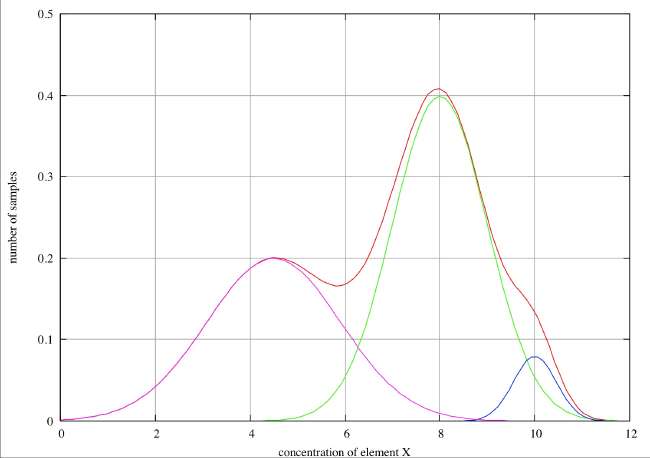
The technique of modal analysis is very simple. We consider all samples together, irrespective of origin, and plot a histogram of frequency of occurrence against (e.g.) concentration of an impurity or trace element. In the following examples we take idealized histograms plotted as continuous distribution functions, and show how they can be broken down into separate normal distributions.
Good Resolution . In this first case we observe two distinct peaks in the histogram and infer that these clearly correspond to two different types of sample, with element ‘X’ concentrations of about 4.2 and 8. We also see a weak, but clear shoulder in the histogram at about 9.8 where there is obviously a point of inflection, and we might reasonably infer that there is a third species with a concentration of about 10. If we have reason to believe that the errors associated with individual species are normally distributed, we can decompose the overall histogram into the individual distributions as shown in the figure.
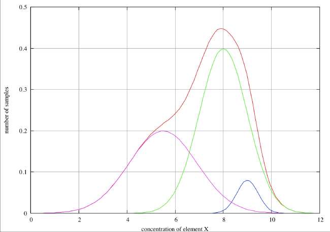
Partial Resolution . In this case we see only a single peak in the histogram with marked broadening on the low concentration side and a point of inflection at about 5.8, and we can reasonably infer two species peaking at about 5.7 and 8. On the high concentration side there is possibly a slight broadening about 8.5, but this is hardly sufficient to infer the presence of a third species. In the case of a real-life, discrete histogram this broadening would not be detectable. If we have reason to believe that the errors associated with individual species are normally distributed, we can decompose the overall histogram into the individual distributions as shown in the figure.
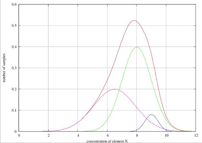
No Resolution . In this case we see only a single peak in the histogram, and although it is very noticeably broadened on the low concentration side, there is no discernible point of inflection and we would not be justified in claiming evidence for more than one species unless we had some hard evidence that the errors were distributed normally. If we had no such evidence, we might speculate that this asymmetry might be the distribution to be expected if there had been a slow drift in concentration over the time period covered by the sample collection. Such an inference would, however, be very speculative.
INAA is generally rather inappropriate for analysis of pottery shards. These are complex mixtures subject to relatively wide variations. It is ideal for monolithic geological samples, jade etc. It is however appropriate for combination with acid extraction.
Acid Extraction is able to identify some (but not all) constituents of shards, but it is, according to Burton and Simon, sensitive enough to distinguish between rather similar cultures. It is also capable of providing confirmation of results from the more subjective morphology approach. I would worry about the possible effect of firing time on acid solubility.
Morphology is suitable for a quick estimate of some constituents of shards, but it is very subjective as applied by Flannery et. al. However, it is essentially a qualitative rather than a quantitative approach: ‘there seems to be quite a lot of something with this crystalline form which appears to me to be the mineral X’.
A more comprehensive approach would be to to submit the same shards to all three techniques: The techniques are complimentary.
A few comments on the application of statistical methods.
Most standard statistical procedures are based upon sampling an unknown distribution, assumed to be ‘normal’. If the unknown distribution is ‘normal’, then, if a sufficiently large sample is considered, the sample mean will approach the true (unknown) mean of the distribution. Experimental errors in making determinations are generally assumed to be distributed normally (theoreticians believe experimentalists have demonstrated this; experimentalists believe theoreticians have established this.) Experimental bias can shift the mean of a normal distribution or distort it from normality (or both.) We need to consider whether samples for analysis have in fact been drawn at random, for example from the total population of pottery shards: if they all come from one small area we suspect bias. We need to consider whether the size of the sample taken is sufficiently large that the mean does approximate the true mean: if the sample size is small the sample mean may differ very significantly from the true mean and generally might possibly invalidate any conclusions.
The first of these worries is susceptible to investigation if the precise location of each shard in a sample has been recorded. In general in an archaeological investigation certain relatively restricted areas receive greater attention. Can these areas be demonstrated to be typical of the whole site?
The second worry is the sample size. To say that a sufficiently large sample size is one which gives (for example) a mean very close to the true (unknown) mean doesn’t help very much. A further complication is that the broader the distribution from which we are drawing a sample, the larger the sample size required to approach the true mean or standard deviation. The trouble is we don’t know the true sample mean or standard deviation, that is what we are trying to find. A realistic approach is to follow the mean and standard deviation as the sample size is increased. We would expect (hope) that these would eventually settle down to a steady value. If, above a certain sample size, the mean and standard deviation do not deviate outside limits which we regard as acceptable, then, providing there is no bias, we might conclude w have found good approximations to true values.
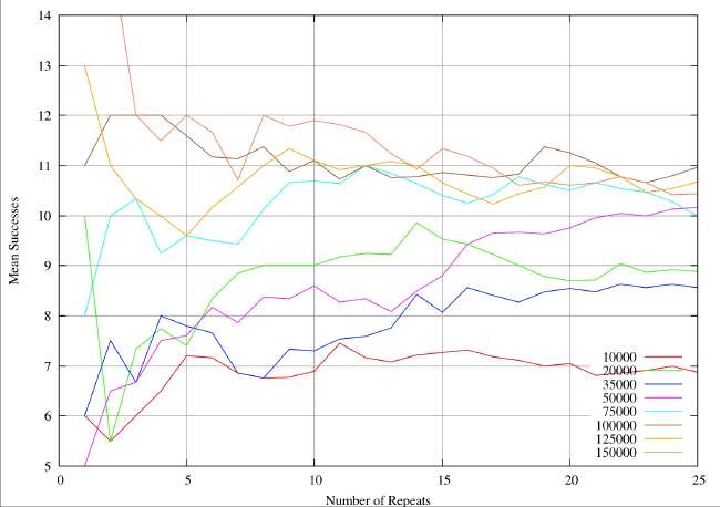
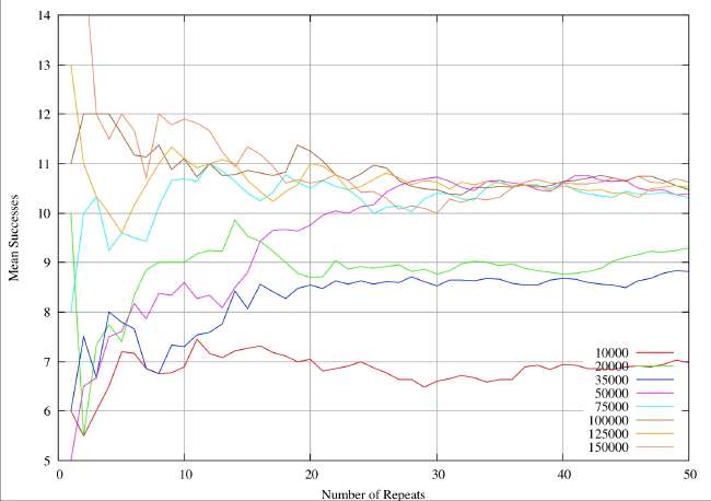
A real-world example can illustrate the sample size problem. These are results from a completely different study (textual analysis of 14th century alliterative poetry), but the statistical analysis and the drawing of conclusions are identical. The distributions are rather broader (30%of the mean) than the ones quoted by Burton and Simon (2.6%), which serves to exaggerate the sample size problem. However, it is very obvious that the sample sizes quoted in table 1 and 2 of Burton and Simon are totally inadequate. In this 14th century example we have eight different subjects of analysis analogous to the different chemical elements. Samples are drawn at random from a distribution known to be normal, each individual instance within a sample corresponding to an individual shard. The sample size is given by the abscissa values (the X-axis) for a continuous variation of sample size. For each sample size the resultant mean is given by the ordinate (Y-value). The plots illustrate the way the sample mean varies with size of sample.
In the first figure, the mean is plotted for sample sizes 1 to 25. Clearly one would be very reluctant to accept any value on the plot as a reasonable approximation to a true mean. Most of the analytical work on shards reported so far is in this range, indeed we have reports of determinations of mean values for sample sizes of 25. Unless the standard deviations of the relevant (unknown) distributions are extremely small I would be very reluctant to draw any conclusions about different origins.
Next we plot the same system for sample values ranging from 1 to 50. It can be seen that the mean values do now appear to settling down, but we would still be very reluctant to accept any value as close to the true mean.
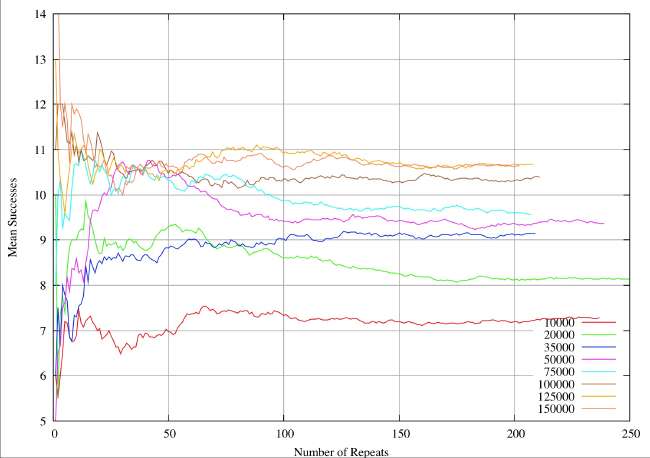
In the next figure we plot the same system for sample sizes ranging from 1 to 250. It now perfectly clear that we are going to see little further change, and we can feel some confidence that we have identified the true mean for the 8 different elements to within about plus or minus 0.05 when we take sample sizes of about 200. For sample sizes of about 150 we have perhaps identified the means to with plus or minus 0.1. In this system, if want reliable statistics we need to take sample sizes of at least 200.
Returning to our pottery shards, we must recognize that we have also chosen to ignore errors originating in the experimental procedures of INAA: someone else has assured us that they are ‘normal’ and ‘sufficiently small’, and that the sample size in the determination is adequately large. (The experimental INAA technique includes the accumulation of repeated measurements on each sample.)
Providing we take adequate precautions about the points outlined above, and are confident that bias has been eliminated or corrected for, we can place considerable confidence in our statistical results.
Generally when we have produced some reliable data we attempt to select a ‘model’ which mimics the data. Often we judge the validity of two or more models by their ability to mimic (‘predict’) the data. If we can build a model which predicts numerical data commensurate with the experimental data, then a usual procedure is to evaluate a chi square statistic for each model and use that to choose the best model. There are limitations to the validity of this procedure (see Catterall and Duddell, NATO Summer School, St. Andrews, 1984 or 5) and other criteria should be applied; the chi square statistic can lead to incorrect evaluation of models.
I believe the low sample sizes quoted in some of the published work hardly justify drawing any conclusions about different sources and origins of pottery shards.
I believe there is a great opportunity to carry out all three techniques on the same samples. The techniques compliment each other.
All the discussion above has been concerned with detecting significant differences in the measured values of a single parameter, such as the concentration of one particular chemical element, in a sample of shards. When we have a multitude of measurable parameters we can reinforce any conclusions by correlations between the distributions of different parameters. If two or more parameters all suggest a similar conclusion our confidence in that conclusion is enhanced. The more parameters that suggest the same conclusion, the stronger our confidence. In figures 4 and 5 of Blomster, Neff and Glascock (BNG) the comparison of tantalum concentrations with chromium and ytterbium agree in that shards from San Lorenzo differ from those from Etlatongo, and that there is some rather weak evidence for a subdivision of Etlatongo into two separate sites. These two analyzes are obviously mutually supportive. Remember we are looking at very minor trace impurities of the order of a few parts per million: a few accidental specks of dust in the mast could completely change the picture.
When we correlate multiple parameters there are problems of representing these in a two or even a three dimensional illustration, and we use a method of factor regression. In figure 1 of Flannery et. al. p. 11220 we see the correlation between the first two factors of Reynolds analysis of the BNG data which account for the bulk of the variations in a total sample size of 184 from 4 different sites. Again we see a grouping into three distinct regions (just possibly four).
My main worry here is that the collection of samples was far from random, they were "selected because they bore the motifs crucial to BNG’s model". This is not simple statistics, this is hypothesis evaluation: we propose a hypothesis (model) that asserts certain motifs are characteristic of a region, and one might reasonably predict from this hypothesis that shards with the same motif should exhibit similarities in trace element concentrations. Reynold’s factor analysis is certainly supportive of this hypothesis. A better approach would have been to take a (much larger) random sample (all the data), and carry out Reynold’s factor analysis. If the same clustering of all samples is observed, then the hypothesis is supported (we know from Reynold’s work that the ‘motif’ samples will cluster). If, however, the inclusion of other samples results in a ‘blurring’, with a more uniform distribution on the scatter plot, then one would begin to suspect the hypothesis and attribute Reynolds analysis to chance.